Solving linear systems¶

Everything above concerns representing and manipulating tensor trains that are already known. This part is about finding one that is not: computing \(x\) from \(A x = b\) with the operator, the right-hand side and the solution all in tensor-train format, and without forming any of them in full.

Three variational solvers are implemented: the one-site Alternating Least Squares (ALS) solver, the two-site Modified Alternating Least Squares (MALS) solver, and the rank-adaptive one-site Alternating Minimal Energy (AMEn) solver. All three sweep over the cores of a tensor train, solving a small projected system at each step; they differ in how many cores that step spans and in how the bond dimensions adapt. See ttnumpy.als(), ttnumpy.mals() and ttnumpy.amen() for the full APIs.

ALS linear solver¶

ttnumpy.als() solves \(A x = b\) by sweeping over single cores. All other cores are held fixed, and the problem restricted to core \(k\) becomes a small linear system:

\[B \, u = b_{loc}, \qquad B = \Psi \cdot A_k \cdot \Phi,\]

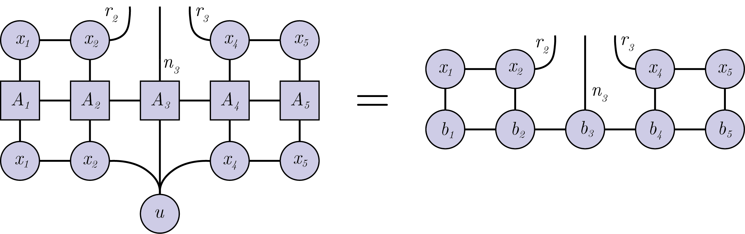
../_images/ALS.png — The one-site ALS system. Contracting the operator with the fixed cores on either side leaves a small problem for the single core \(u\).¶

where \(\Psi\) and \(\Phi\) are the left and right environments. The solution \(u\) replaces core \(k\) as a whole. It is then orthogonalized by a QR factorization whose triangular factor is absorbed by the neighbouring core, which moves the orthogonality centre one site along and leaves the represented tensor unchanged.

Fixed ranks by construction¶

A one-site step replaces a core without ever splitting a bond, so ALS cannot increase the bond dimensions. The solution is sought inside the fixed-rank manifold of the initial guess, which means x0 must already carry enough rank to represent the answer. (Ranks may still shrink: the economic QR removes a bond that exceeds what its neighbouring core can support.)

The upside is cost. A one-site system has \(r_{k-1} \cdot n_k \cdot r_k\) unknowns against the \(r_{k-1} \cdot n_k \cdot n_{k+1} \cdot r_{k+1}\) of a MALS supercore — smaller by roughly a factor of mode size times rank — so the direct solve on the explicit matrix stays affordable to much larger problems.

The downside is stagnation. Given a rank-deficient guess, ALS has no mechanism to escape, and sweeping simply stalls above the target tolerance. On the 1D QTT Laplacian of order 6, whose solution is a parabola of exact TT rank 3, this is sharp:

Guess rank	`stop_reason`	Final residual
1	`stagnated`	5.6e+00
2	`stagnated`	1.0e+00
3	`converged`	1.5e-13
6	`converged`	2.8e-13

Removing exactly this failure mode — while keeping the cheap one-site local system — is what the residual enrichment of AMEn linear solver below is designed for.

Stopping¶

residual_tol sets the target for the relative residual \(\|Ax - b\| / \|b\|\), measured in TT arithmetic after every sweep, and also fixes the tolerance of the iterative local solves. As in MALS, stop_reason is "converged", "stagnated" or "max_sweeps", and return_info=True returns the record as a ttnumpy.SolverInfo. Since ALS has no truncation to control, residual_tol is its only accuracy parameter; the local solvers described below behave exactly as they do for MALS.

Example¶

import ttnumpy as tt

# the guess fixes the ranks for the whole run, so give it enough
x0 = tt.ones(b.physical_dims(), ranks=8).compress_svd(canonical="right")

x, info = tt.als(
    A,                    # TTM operator
    b,                    # TT right-hand side
    x0=x0,
    residual_tol=1e-8,
    max_sweeps=10,
    symmetric=True,
    return_info=True,
)
print(info.stop_reason, info.residuals[-1])

Omitting x0 starts from an all-ones train with the ranks of b, which is only adequate when the solution is no richer than the right-hand side.

MALS linear solver¶

ttnumpy.mals() solves \(A x = b\) with the operator A given as a TT-matrix and b, x as tensor trains. The implementation follows the DMRG-type scheme of Oseledets and Dolgov [OD2012].

One sweep runs over all pairs of neighbouring cores. For each pair, all other cores are held fixed and the problem restricted to that pair becomes a small linear system:

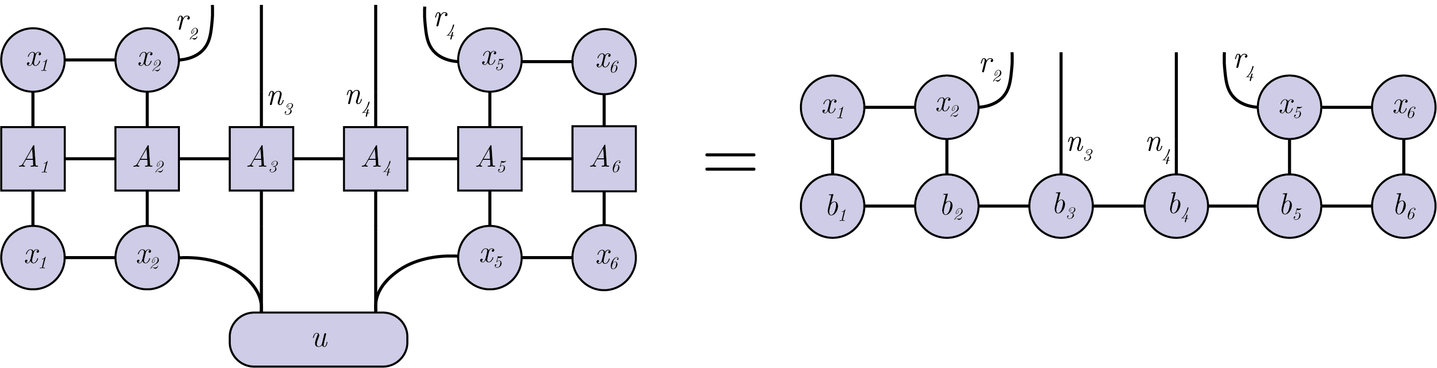
\[B \, u = b_{loc}, \qquad B = \Psi \cdot A_k \cdot A_{k+1} \cdot \Phi,\]

../_images/MALS.png — The two-site MALS system. The unknown is the supercore \(u\) spanning two physical indices, which is split by an SVD once solved.¶

where \(\Psi\) and \(\Phi\) are the left and right environments, same as in ALS (contractions of A with the fixed cores of x, eq. (3.11) of [OD2012]). The solution \(u\) is split back into two cores by an SVD, which is also where the bond dimension adapts: the number of singular values kept sets the new rank.

Accuracy control¶

The recommended way to control accuracy is the residual_tol parameter, the target for the relative residual \(\|Ax - b\| / \|b\|\). It drives both the truncation and the stopping criterion:

Truncation (trick 2, section 4.2 of [OD2012]): each SVD keeps the smallest rank whose local residual stays within budget, so ranks grow exactly as far as the target requires.
Stopping: the global relative residual is measured after every sweep in TT arithmetic (nothing is densified). The solver returns with stop_reason equal to "converged", "stagnated" (a sweep improved the residual by less than stagnation_factor), or "max_sweeps". Pass return_info=True to receive this record as a ttnumpy.SolverInfo.

Without residual_tol, truncation falls back to discarding singular values below error_threshold relative to the largest one. Note that this bounds the error of the solution, while the residual may stay as large as \(\mathrm{cond}(A) \cdot\) error_threshold — for ill-conditioned operators such as discretized Laplacians this floor is substantial. error_threshold mode is recommended only for well-conditioned operators, when the perofrmace is the priority.

Local solvers¶

Small local systems are solved by LU on the explicit matrix. Once a system exceeds direct_solve_size unknowns (possible at bond dimensions above roughly 15), forming and factorizing that matrix costs like \(~\mathcal{O}(r^6)\). In that regime the solver switches to a matrix-free Krylov method: the local operator is applied as a chain of small tensor contractions (section 3.4 of [OD2012]), and the iteration is warm-started from the current supercore (trick 1, section 4.1 of [OD2012]).

The Krylov iteration is held to local_rtol. Left unset, that is a tenth of residual_tol when one is given and a fixed default otherwise, so the dispatch does not depend on which accuracy parameters are in use — only on local_solver and direct_solve_size.

A local solve that misses its tolerance is accepted as it stands. The sweep is self-correcting, so this normally costs iterations rather than accuracy, and it keeps the peak memory bounded by direct_solve_size. Passing allow_dense_fallback=True instead redoes such a solve exactly on the explicit matrix: local solves are then always as accurate as requested, at the price of building the very matrix the matrix-free path avoids — at max_rank=50 that is a 0.8 GB operator. Prefer it only when the inexact solves are demonstrably holding the sweep back; SolverInfo reports local_fallbacks and local_inexact so the choice can be checked rather than guessed.

For symmetric operators pass symmetric=True so that MINRES is used; otherwise GMRES is chosen, which on a symmetric operator is the more expensive way to get the same answer. local_solver="direct" disables the iterative path entirely.

Example¶

import ttnumpy as tt

x, info = tt.mals(
    A,                    # TTM operator
    b,                    # TT right-hand side
    residual_tol=1e-6,    # target relative residual
    max_sweeps=15,
    symmetric=True,       # e.g. a discretized Laplacian
    return_info=True,
)
print(info.stop_reason, info.residuals[-1])

A "stagnated" result above the requested tolerance means the sweeping scheme cannot make further progress at the current settings; plain MALS carries no convergence guarantee for such cases (section 4.3 of [OD2012] discusses restarts, and residual-enriched methods such as AMEn address it systematically).

AMEn linear solver¶

ttnumpy.amen() keeps the one-site local system of ALS but makes the ranks adapt, following Dolgov and Savostyanov [DS2014]. For an SPD system the gradient of the energy

\[J(x) = \tfrac12 x^\top A x - x^\top b\]

is \(\nabla J = Ax - b\), so the residual \(r = b - Ax\) is the steepest-descent direction. After solving core \(k\), AMEn appends an approximation of that direction to the core, which enlarges the subspace the next local solve explores.

../_images/AMEN.png — An AMEn step: the solved core \(u_1\) is augmented with the residual direction \(z_1\), widening the bond for the next local solve.¶

The enrichment does not change the represented solution. Extra columns are appended to core \(k\) along the bond facing the sweep direction, and the neighbouring core is padded with matching zero rows, so the appended directions contribute nothing until the next solve fills them in.

The residual train¶

The exact residual is unusable as an enrichment: in TT format \(b - Ax\) has rank \(r_b + r_A r_x\), which would multiply the solution’s rank at every step. AMEn instead carries a separate train \(z \approx b - Ax\) of rank kickrank (2–4 is typical), refitted core by core as the sweep proceeds so that it tracks the solution as it changes.

Refitting \(z\) is cheap. It is a least-squares fit rather than a linear system, and with the surrounding cores of \(z\) orthonormal the optimal core is just the projection of \(b - Ax\) onto that frame — no local system is solved.

Before it can be appended, \(z\)’s core has to be expressed in the frame of \(x\), because the two trains carry different bond bases. Write \(X_{<k}\) for the left interface matrix of \(x\) at bond \(k\): the first \(k\) cores contracted and reshaped to \((n_0 \cdots n_{k-1}) \times r_k\), whose columns are orthonormal once the sweep has passed them. With \(Z_{<k}\) the same object built from \(z\), the change of basis is their overlap, and applying it amounts to an orthogonal projection:

\[X_{<k}^{\dagger} Z_{<k} \in \mathbb{C}^{r_k \times \rho_k}, \qquad X_{<k} \left( X_{<k}^{\dagger} Z_{<k} \right) = P_x \, Z_{<k}, \quad P_x = X_{<k} X_{<k}^{\dagger}.\]

Note this is a matrix, not a scalar — the contraction runs over the first \(k\) cores only, not the whole train. Appending \(\left( X_{<k}^{\dagger} Z_{<k} \right) z_k\) therefore adds the part of the residual direction that the frozen left cores can actually represent. The component outside that subspace is recovered at other sites as the sweep moves on. The backward sweep uses the right interfaces \(X_{>k}\) and \(Z_{>k}\) in the same way.

Rank control¶

Each solved core is SVD-truncated before the enrichment is appended: singular values below error_threshold relative to the largest are dropped, and max_rank caps the result. A bond therefore ends each step at the rank the accuracy budget requires plus at most kickrank, instead of growing by kickrank on every visit. Because the enrichment is added on top of the truncated core, bonds may exceed max_rank by up to kickrank.

Set error_threshold at or below the accuracy actually wanted — roughly residual_tol / 10 is a reasonable default. A threshold that is too loose truncates away the progress the enrichment just bought.

Example¶

import ttnumpy as tt

x, info = tt.amen(
    A,                     # TTM operator
    b,                     # TT right-hand side
    x0=None,               # initial guess
    kickrank=3,            # rank of the residual train
    error_threshold=1e-10,
    residual_tol=1e-8,
    max_sweeps=20,
    symmetric=True,
    return_info=True,
)
print(info.stop_reason, info.residuals[-1], info.max_bonds)

x0 is accepted here exactly as it is by the other two solvers, but AMEn is the one that rarely needs it. Left unset it defaults to an all-ones train with the ranks of b, and unlike ALS a poor guess costs nothing — the enrichment builds up whatever rank the solution requires as the sweep proceeds.

info.max_bonds records the largest bond dimension after each sweep, which is the quickest way to see the rank adaptation at work.

Choosing a solver¶

All three share the environments, the local solvers and the stopping machinery; the choice is about rank adaptation.

Use AMEn as the default for large problems. It adapts the ranks from any starting guess, its one-site local systems stay small, and the residual enrichment gives it a convergence guarantee for SPD systems that neither of the others has. On the order-6 QTT Laplacian above, where ALS stagnates at a residual of 5.6 from a rank-1 guess, AMEn reaches \(10^{-13}\) from the same guess.

Use MALS when the mode sizes are small and the rank profile varies sharply from bond to bond: the two-site SVD adapts each bond in one shot, rather than a few units per sweep, and residual_tol alone controls both accuracy and rank growth. Its residual-based truncation is also the more refined of the two truncation schemes implemented here.

Use ALS when the rank is already known or deliberately fixed: refining a solution obtained elsewhere, re-solving a problem whose rank profile is known from a previous run, or working under a hard memory budget where ranks must not grow at all.

Note that a "stagnated" result means different things. For MALS and AMEn it indicates the sweeping scheme itself has stalled; for ALS it usually just means the guess had too little rank, and retrying with a richer x0 — or switching to AMEn — is the first thing to try.

References¶

[OD2012] (1,2,3,4,5,6)

I. V. Oseledets and S. V. Dolgov, Solution of linear systems and matrix inversion in the TT-format, SIAM J. Sci. Comput. 34(5), A2718–A2739, 2012. https://doi.org/10.1137/110833142

[DS2014]

S. V. Dolgov and D. V. Savostyanov, Alternating minimal energy methods for linear systems in higher dimensions, SIAM J. Sci. Comput. 36(5), A2248–A2271, 2014. https://doi.org/10.1137/140953289